Chapters 1-3 Notes
Grid Approximation
# Step 1: Define the grid, what are all the values you're going to consider
p_grid <- seq(from=0, to=1, length.out = 1000)

# Step 2: Define the prior: Assume uniform and assign 1 to every value of p we're considering. We assign 1 so that the integral sums to 1
prob_p <- rep(1, 1000)

# Step 3: Get the probability of the data, aka, the likelihood. 6 waters, 9 tosses
prob_data <- dbinom(6, size=9, prob=p_grid)

# Step 4: Computer the posterior
posterior <- prob_data * prob_p

# Step 5: Standardize the posterior
posterior <- posterior / sum(posterior)

plot(p_grid, posterior, type = "b",
     xlab = "probability of water",
     ylab = "posterior probability")
mtext("1000 points")
Quadratic Approximation
# Step 1: Find the posterior mode.
# Step 2: Once you find the peak of the posterior, estimate the curvature near the peak
# note map() stands for maximum a posteriori aka, the mode of the posterior

library(rethinking)
globe.qa <- map(
  alist(
    w ~ dbinom(9,p), # binomial likelihood
    p ~ dunif(0,1) # uniform prior
  ),
  data = list(w=6))

# display summary of quadratic approximation
# Interpretation: assuming the posterior is Gaussian, it is maximized at 0.67, and its
# standard deviation is 0.16
precis(globe.qa)
## mean sd 5.5% 94.5%
## p 0.6666665 0.1571338 0.4155363 0.9177967Sampling
In order to pull samples we need a posterior to pull from. We’ll reuse the grid approximation from the globe tossing example.
p_grid <- seq(0, 1, length.out = 1000)
prior <- rep(1, 1000)
likelihood <- dbinom(6, size = 9, prob = p_grid)
posterior <- likelihood * prior
posterior <- posterior/sum(posterior)
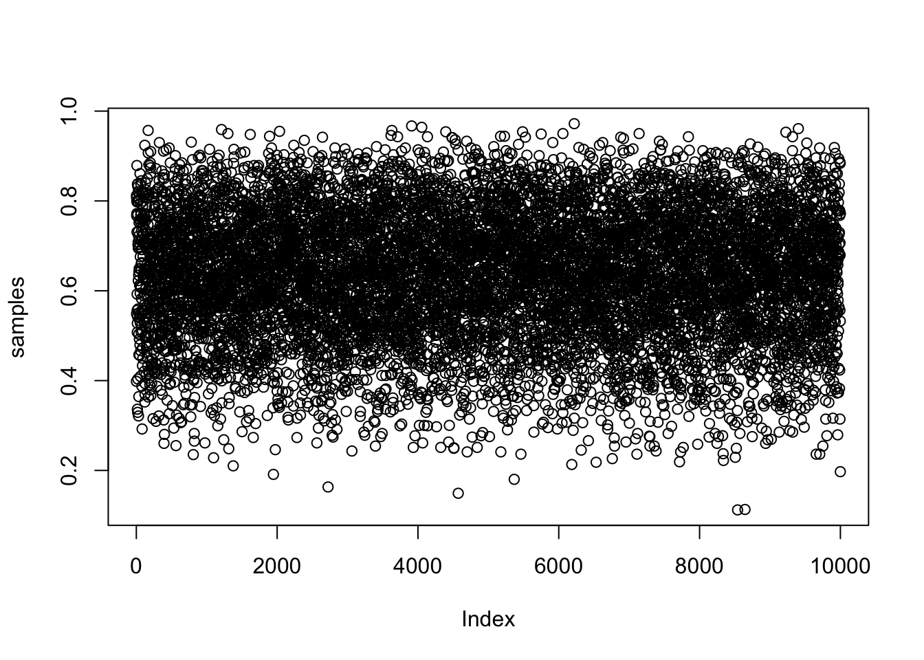
Now assume we want to draw 10,000 samples from this posterior
samples <- sample(p_grid, prob = posterior, size = 1e4, replace = TRUE)
plot(samples)
As we can see below, the estimated density of our samples is very similar to our posterior. As we draw more samples it will get more and more similar
dens(samples)
plot(posterior)
Intervals of defined boundary
Suppose we want the probability that the proportion of water is less than 0.5.
sum(posterior[p_grid < 0.5])## [1] 0.1718746We can perform this same calculation using the samples from the posterior too.
sum(samples < 0.5)/1e4## [1] 0.1696Intervals of defined mass
These are usually known as confidence intervals. These intervals report two parameter values that contain between them a specified amount of posterior probability, a probability mass.
If we wanted the lower 80% we could run the code below and see that posterior probability exists below a parameter value of about 0.76.
quantile(samples, 0.8)## 80%
## 0.7607608Similarly if we wanted the middle 80% interval
quantile(samples, c(0.1, 0.9))## 10% 90%
## 0.4493493 0.8128128However we must be careful. These intervals, which we’ll call percentile intervals (PI), assign an equal probability mass to each tail. They do a good job of communitcating the shape of a distribution, as long as the distribution isn’t too asymetrical. The highest posterior density interval (HPDI) is the narrowest interval containing the specified probability mass.
Let’s consider an example to illustrate the difference. If we toss a globe three times and it lands on water every time, we’ll see that PI excludes the most probable parameter values, near \(p = 1\).
p_grid <- seq(0, 1, length.out = 1000)
prior <- rep(1, 1000)
likelihood <- dbinom(3, size = 3, prob = p_grid)
posterior <- likelihood * prior
posterior <- posterior/sum(posterior)
samples <- sample(p_grid, size = 1e4, replace = TRUE, prob = posterior)
Visually we can see that HPDI is narrower, but we can also calculate this below to see that HPDI has a width of about 0.16 in comparison to 0.22 for the percentile interval.
PI_interval <- PI(samples, prob = 0.5)
HPDI_interval <- HPDI(samples, prob = 0.5)

PI_interval[[2]] - PI_interval[[1]]
## [1] 0.2242242HPDI_interval[[2]] - HPDI_interval[[1]]## [1] 0.1591592HPDI has some advantages over the PI, but in most cases, these two types of interval are very similar. When the posterior is bell shaped, it hardly matters which type of interval you use.
It’s also important to realize that HPDI does have some disadvantages. HPDI is more computationally intensive than PI and suffers from greater simulation variance meaning that it is sensitive to how many samples you draw from the posterior.
Point Estimates
Given the entire posterior distribution, what value should you report? Let’s reuse the previous example, of observing three waters out of three tosses. We’l consider three examples.
First we’ll look at the parameter value with the highest posterior probability.
p_grid[which.max(posterior)]## [1] 1Or if we have samples from the posterior, we can still approximate the same point.
# chainmode returns the estimated mode of a density computed from samples
chainmode(samples, adj = 0.01)
## [1] 0.9955165One way we can go beyond using the entire posterior as the estimate is to choose a loss function. The important thing to understand is that different loss functions imply different point estimates.
Here we see that using an absolute loss function is equivalent (up to sampling variance) to the median. The quadratic loss \((d - p)^2\) is another common loss function, which leads to the posterior mean i.e. mean(samples) as the point estimate.
loss <- sapply(p_grid, function(d) sum(posterior*abs(d-p_grid)))
p_grid[which.min(loss)]
## [1] 0.8408408median(samples)## [1] 0.8408408Dummy Data
Bayesian models are always generative, meaning that they’re capable of simulating predictions. We call such simulated data, dummy data. If we wanted to simulate observations for our globe tossing experiment we can use the rbinom() function in r. Let’s say we want to generate 100,000 dummy observations. Notice how this is nearly identical to the analytical approach.
| Generated | Analytical | |
|---|---|---|
| 0 | 0.08914 | 0.09 |
| 1 | 0.42273 | 0.42 |
| 2 | 0.48813 | 0.49 |
Model Checking
Model checking means (1) ensuring the model fitting worked correctly and (2) evaluating the adequacy of a model for some purpose.